Prolog Factor Language

Introduction

The package also includes implementations for a set of well-known inference algorithms for solving probabilistic queries on these models. Both ground and lifted inference methods are support.

Back to the top

Installation

In case you want to install YAP somewhere else or with different settings, please consult the YAP documentation. From now on, we will assume that the directory $HOME ▷ bin (where the binary is) is in your $PATH environment variable.

Once in a while, we will refer to the PFL examples directory. In a default installation, this directory will be located at $HOME ▷ share ▷ doc ▷ Yap ▷ packages ▷ examples ▷ CLPBN.

Back to the top

Language

• Type refers the type of network over which the parfactor is defined. It can be bayes for directed networks, or markov for undirected ones.

• F is a comma-separated sequence of Prolog terms that will define sets of random variables under the constraint C. If Type is bayes, the first term defines the node while the remaining terms define its parents.

• Phi is either a Prolog list of potential values or a Prolog goal that unifies with one. Notice that if Type is bayes, this will correspond to the conditional probability table. Domain combinations are implicitly assumed in ascending order, with the first term being the 'most significant' (e.g. x₀y₀, x₀y₁, x₀y₂, x₁y₀, x₁y₁, x₁y₂).

• C is a (possibly empty) list of Prolog goals that will instantiate the logical variables that appear in F, that is, the successful substitutions for the goals in C will be the valid values for the logical variables. This allows the constraint to be defined as any relation (set of tuples) over the logical variables.

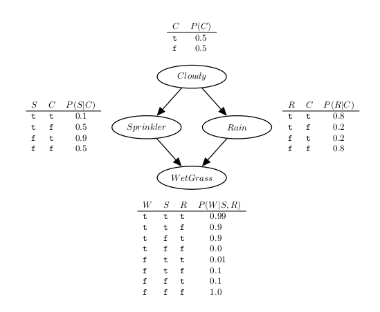
Towards a better understanding of the language, next we show the PFL representation for the sprinkler network found in the above figure.

:- use_module(library(pfl)).

bayes cloudy ; cloudy_table ; [].

bayes sprinkler, cloudy ; sprinkler_table ; [].

bayes rain, cloudy ; rain_table ; [].

bayes wet_grass, sprinkler, rain ; wet_grass_table ; [].

cloudy_table(
    [ 0.5,
      0.5 ]).

sprinkler_table(
    [ 0.1, 0.5,
      0.9, 0.5 ]).

rain_table(
    [ 0.8, 0.2,
      0.2, 0.8 ]).

wet_grass_table(
    [ 0.99, 0.9, 0.9, 0.0,
      0.01, 0.1, 0.1, 1.0 ]).

In the example, we started by loading the PFL library, then we have defined one factor for each node, and finally we have specified the probabilities for each conditional probability table.

Notice that this network is fully grounded, as all constraints are empty. Next we present the PFL representation for a well-known markov logic network - the social network model. For convenience, the two main weighted formulas of this model are shown below.

1.5 : Smokes(x) => Cancer(x)
1.1 : Smokes(x) ^ Friends(x,y) => Smokes(y)

Next, we show the PFL representation for this model.

:- use_module(library(pfl)).

person(anna).
person(bob).

markov smokes(X), cancer(X) ;
    [4.482, 4.482, 1.0, 4.482] ;
    [person(X)].

markov friends(X,Y), smokes(X), smokes(Y) ;
    [3.004, 3.004, 3.004, 3.004, 3.004, 1.0, 1.0, 3.004] ;
    [person(X), person(Y)].

Notice that we have defined the world to be consisted of only two persons, anna and bob. We can easily add as many persons as we want by inserting in the program a fact like person @ 10. . This would automatically create ten persons named p1, p2, ..., p10.

Unlike other fist-order probabilistic languages, in PFL the logical variables that appear in the terms are not directly typed, and they will be only constrained by the goals that appears in the constraint of the parfactor. This allows the logical variables to be constrained to any relation (set of tuples), and not only pairwise (in)equalities. For instance, the next example defines a network with three ground factors, each defined respectively over the random variables p(a,b), p(b,d) and p(d,e).

constraint(a,b).
constraint(b,d).
constraint(d,e).

markov p(A,B); some_table; [constraint(A,B)].

We can easily add static evidence to PFL programs by inserting a fact with the same functor and arguments as the random variable, plus one extra argument with the observed state or value. For instance, suppose that we know that anna and bob are friends. We can add this knowledge to the program with the following fact: friends(anna,bob,t). .

One last note for the domain of the random variables. By default, all terms instantiate boolean (t/f) random variables. It is possible to choose a different domain for a term by appending a list of its possible values or states. Next we present a self-explanatory example of how this can be done.

bayes professor_ability::[high, medium, low] ; [0.5, 0.4, 0.1].

More probabilistic models defined using PFL can be found in the examples directory.

Back to the top

Querying

Assuming that the current directory is the one where the examples are located, first we load the model with the following command.

$ yap -l sprinkler.pfl

Let's suppose that we want to estimate the marginal probability for the WetGrass random variable. To do so, we call the following goal.

?- wet_grass(X).

The output of this goal will show the marginal probability for each WetGrass possible state or value, that is, t and f. Notice that in PFL a random variable is identified by a term with the same functor and arguments plus one extra argument.

Now let's suppose that we want to estimate the probability for the same random variable, but this time we have evidence that it had rained in the day before. We can estimate this probability without resorting to static evidence with:

?- wet_grass(X), rain(t).

PFL also supports calculating joint probability distributions. For instance, we can obtain the joint probability for Sprinkler and Rain with:

?- sprinkler(X), rain(Y).

Back to the top

Options

• ve, variable elimination (written in Prolog)
• hve, variable elimination (written in C++)
• jt, junction tree
• bdd, binary decision diagrams
• bp, belief propagation
• cbp, counting belief propagation
• gibbs, gibbs sampling
• lve, generalized counting first-order variable elimination (GC-FOVE)
• lkc, lifted first-order knowledge compilation
• lbp, lifted first-order belief propagation

For instance, if we want to use belief propagation to solve some probabilistic query, we need to call first:

?- set_solver(bp).

It is possible to tweak some parameters of PFL through set_pfl_flag/2 predicate. The first argument is a option name that identifies the parameter that we want to tweak. The second argument is some possible value for this option. Next we explain the available options in detail.

verbosity

• Values: a positive integer (default is 0 - no debugging). The higher the number, the more information that will be shown.
• Affects: hve, bp, cbp, lve, lkc and lbp.

For instance, we can view some basic debugging information by calling the following goal.

?- set_pfl_flag(verbosity, 1).

use_logarithms

• Values: true (default) or false.
• Affects: hve, bp, cbp, lve, lkc and lbp.

hve_elim_heuristic

• Values: sequential, min_neighbors, min_weight, min_fill and
  weighted_min_fill (default).
• Affects: hve.

An explanation for each of these heuristics can be found in Daphne Koller's book Probabilistic Graphical Models.

bp_max_iter

• Values: a positive integer (default is 1000).
• Affects: bp, cbp and lbp.

bp_accuracy

• Values: a float-point number (default is 0.0001).
• Affects: bp, cbp and lbp.

bp_msg_schedule

• Values:
  • seq_fixed (default), at each iteration, all messages are sent with the same order.

  • seq_random, at each iteration, all messages are sent with a random order.

  • parallel, at each iteration, all messages are calculated using only the values of the previous iteration.

  • max_residual, the next message to be sent is the one with maximum residual (as explained in the paper Residual Belief Propagation: Informed Scheduling for Asynchronous Message Passing).
• Affects: bp, cbp and lbp.

export_libdai

• Values: true or false (default).
• Affects: hve, bp, and cbp.

export_uai

• Values: true or false (default).
• Affects: hve, bp, and cbp.

export_graphviz

• Values: true or false (default).
• Affects: hve, bp, and cbp.

print_fg

• Values: true or false (default).
• Affects: hve, bp, and cbp.

Back to the top

Learning

Next we show an example of parameter learning for the sprinkler network.

:- [sprinkler.pfl].

:- use_module(library(clpbn/learning/em)).

data(t, t, t, t).
data(_, t, _, t).
data(t, t, f, f).
data(t, t, f, t).
data(t, _, _, t).
data(t, f, t, t).
data(t, t, f, t).
data(t, _, f, f).
data(t, t, f, f).
data(f, f, t, t).

main :-
    findall(X, scan_data(X), L),
    em(L, 0.01, 10, CPTs, LogLik),
    writeln(LogLik:CPTs).

scan_data([cloudy(C), sprinkler(S), rain(R), wet_grass(W)]) :-
    data(C, S, R, W).

Parameter learning is done by calling the em/5 predicate. Its arguments are the following.

• Data is a list of samples for the distribution that we want to estimate. Each sample is a list of either observed random variables or unobserved random variables (denoted when its state or value is not instantiated).
• MaxError is the maximum error allowed before stopping the EM loop.
• MaxIters is the maximum number of iterations for the EM loop.
• CPTs is a list with the estimated conditional probability tables.
• LogLik is the log-likelihood.

It is possible to choose the solver that will be used for the inference part during parameter learning with the set_em_solver/1 predicate (defaults to hve). At the moment, only the following solvers support parameter learning: ve, hve, bdd, bp and cbp.

Inside the learning directory from the examples directory, one can find more examples of parameter learning.

Back to the top

External Interface

This command's name is hcli and its usage is as follows.

$ ./hcli [solver=hve|bp|cbp] [<OPTION>=<VALUE>]... <FILE>[<VAR>|<VAR>=<EVIDENCE>]...

Let's assume that the current directory is the one where the examples are located. We can perform inference in any supported model by passing the file name where the model is defined as argument. Next, we show how to load a model with hcli.

$ ./hcli burglary-alarm.uai

With the above command, the program will load the model and print the marginal probabilities for all defined random variables. We can view only the marginal probability for some variable with a identifier X, if we pass X as an extra argument following the file name. For instance, the following command will output only the marginal probability for the variable with identifier 0.

$ ./hcli burglary-alarm.uai 0

If we give more than one variable identifier as argument, the program will output the joint probability for all the passed variables.

Evidence can be given as a pair containing a variable identifier and its observed state (index), separated by a '=`. For instance, we can introduce knowledge that some variable with identifier 0 has evidence on its second state as follows.

$ ./hcli burglary-alarm.uai 0=1

By default, all probability tasks are resolved using the hve solver. It is possible to choose another solver using the solver option as follows.

$ ./hcli solver=bp burglary-alarm.uai

Notice that only the hve, bp and cbp solvers can be used with hcli.

The options that are available with the set_pfl_flag/2 predicate can be used in hcli too. The syntax is a pair <Option>=<Value> before the model's file name.

Back to the top

Papers

• Evaluating Inference Algorithms for the Prolog Factor Language.

Back to the top